New Products

xpswmm 2011 Runoff analysis, flood analysis software Price:693,000 Yen (New purchase) Release:October 2011 Water works

Design Festival 2011-3Days November 15, 2011:VRcon.forum8.jp November 16 and 17: Shinagawa front building Day3 "Water works" Session xpswmm user meeting CPD Certificate November 17, 2011 13:00-12:00 Meeting room B

Release of xpswmmj 2011

"xpswmmj 2011" in Japanese is renewed. In this year, xpswmm2D (xp2d module) is approved by the United States Federal emergency Management Agency (FEMA) for two-dimensional flood modeling and mapping for the National Flood Insurance Program (NFIP9). In the latest version, 2D analysis function including multiple 2D domain as an add-on module is enhanced. Please try to use the world latest runoff analysis and flood analysis with the latest version.

New features

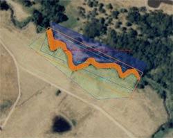
The new functions in this version up are as follow: Multiple 2D domain Dual drainage batch converter Optimization function of reservoir Calculation of the concentrated time under hydrological analysis Output of flow velocity and flow velocity vector in a location Improved import function of the external data The new functions of the latest version are as follows. Add-on module 1.Multiple 2D domain The multiple 2D domain allows the setting of the cell size and the multiple grid ranges in different directions (Figure 1). With this function, the diversity of the surface flow modeling can be supported and the analysis accuracy can be improved. For example, the smaller size of cell is specified for the complex geographical area, the open channel such as rivers, the urban area where there are many structures which may block that flow, and the larger size of cell is specified for the simple and plane ground. In addition, the grid direction can be easily changed to fit in with the exhaustive terrain which has the flow direction such as railway and river channel. Figure1 Setting of multiple grid ranges In the boundary part of the different grid range, the calculation and visualization can be seamlessly performed by the new attribution 2D/2D interface which consists of polyline (Figure2). 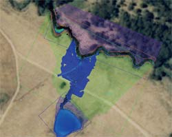Figure 2 Setting of 2D/2D interface The flow from a 2D domain is run off continuously via 2D/2D interface as the water level and flow rate are sequentially linked between different 2D domains via 2D/2D interface (Figure 3). Figure 3 Analysis result of modeling with multiple 2D domain The high-accurate analysis can be performed in the entire area of 2D analysis, and the number of cells of 2D analysis can be reduced by setting the rough cell size in the plane part so that the analysis speed is expected to be improved. For example, 2m cell size is applied to the river channel along the narrow river, and the city area where there are many houses can be modeled with 5m mesh and the plane ground can be modeled with 10m mesh (Figure 4). Figure 4 Analysis example with multiple 2D domain Updated function 2. Dual drainage batch converter The modeling of the flood analysis under one dimension analysis is the manual method which causes the error where it takes too much time for converting from the single link to multiple links (Figure5). Figure 5 One dimension flood analysis model where the surface flow is represented by the road sandwiched between edge stones From this version, this automation replaces a time-consuming and error prone manual task to convert single conduits for dual drainage (Figure6).  Figure 6 Flow of convert to road surface flow model 3.Optimization function of reservoir The optimization functions of the reservoir are updated and enhanced in four types of automatic design options. The size of node and link is automatically optimized by the option which defines the maximum water level of the downstream pipe, the maximum water level of the reservoir, the maximum water level of both (Table 1). Table 1 Optimization option of reservoir Optimization option Contents of automatic process Resize of downstream pipe The downstream pipe is enlarged not to exceed the maximum water level required in the reservoir. Resize of reservoir amount When it exceeds the maximum water level of the reservoir (hydraulic-grade line), the reservoir capacity is changed. The algorithm with this method is used in the two steps: Exponential search stage and fine-adjustment stage Limit of flow amount of downstream pipe When the predefined maximum flow rate is exceeded, the size of downstream pipe is reduced. Resize of downstream pipe and reservoir amount The reservoir capacity is defined by the existing downstream pipe. When the reservoir capacity which satisfies these conditions is available, the flow rate in the downstream pipe is checked. When it exceeds the flow rate in the downstream, the pipe diameter is reduced and the reservoir capacity is calculated again. 4.Calculation of the concentrated time under hydrological analysis The calculation of the concentrated time/concentrated time to peak can be performed not only with time area method but 9 types of methods (Friend's Equation, Modified Friend Formula, Kinematic Wave, Alameda, Izzard, Kerby, Kirpich, Federal Aviation Authority, and Bransby Williams) with "SCS(US Soil Conservation Service)" and "Unit hydrograph method" (Figure7, 8). 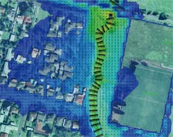Figure 7 Calculation of concentrated time with SCS hydrological method Figure 8 Calculation of concentrated time with unit hydrograph method 5.Output of flow velocity and flow velocity vector in a location Time-historical result of water level, flow velocity, and flow direction under 2D analysis in an arbitrary location is output(Figure 9). Figure 9 Time-historical output of flow velocity and flow velocity vector in a location 6.Improved import function of the external data Import of 2D grid area The import of 2D grid area in GIS format (Shape file and MapInfo file) is now supported. Export of flow rate and flow velocity vector The 2D vector layer can be exported in ESRI grid file format while mapping the flow rate and flow velocity vector. Attribution import while importing the node and link from GIS file The import of the shape with the attribution while importing the node and link from GIS file is now supported.

(Up&Coming '11 Late fall issue)